정확도(Precision), 재현율(Recall)과 참고사항
이해하기 쉽고, 장황하지 않은 자료를 기반으로 강의를 진행합니다.
8. 정확도(Precision), 재현율(Recall)과 참고사항
- 정확도: 검색 결과로 가져온 문서 중 실제 관련된 문서 비율
- 재현율: 관련 문서 중 검색된 문서 비율
- 예
- 100개 문서를 가진 검색엔진에서
- '범죄도시' 라는 키워드로 검색시, 검색 결과로 20개 문서가 나온 경우
- 이 때 20개 문서 중 16개 문서가 실제 '범죄도시' 와 관련된 문서이고
- 전체 100개 문서 중 '범죄도시' 와 관련된 총 문서는 32개라고 하면
- 정확도: 16 / 20 = 0.8
- 재현율: 16 / 32 = 0.5
- 100개 문서를 가진 검색엔진에서
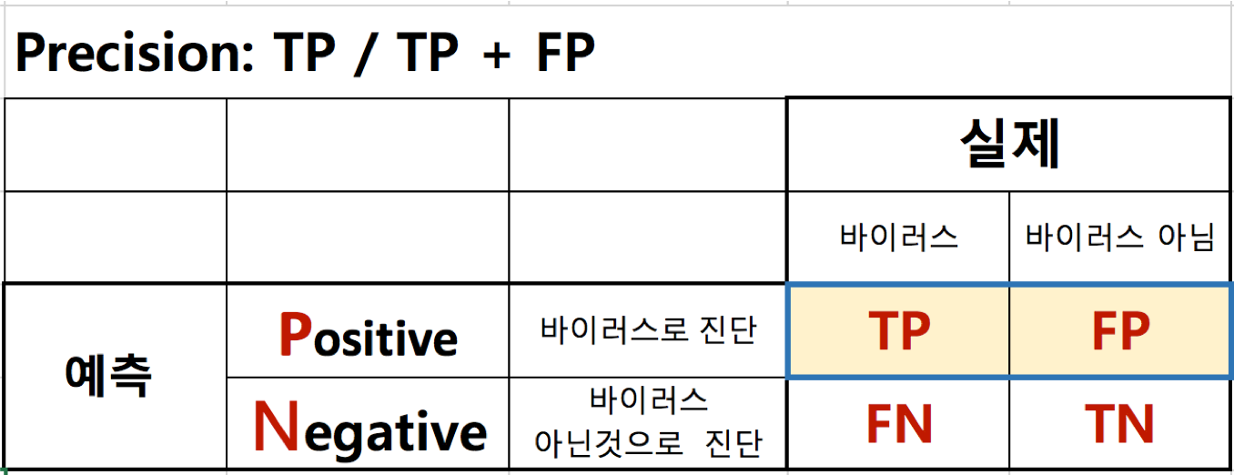
- TP(True Positive)는 추천된 항목이 사용자가 선호하는 항목인 개수
- FP(False Positive)는 추천된 항목이 사용자가 선호하지 않는 항목인 개수
- FN(False Negative)은 추천되지 않았지만 사용자가 선호하는 항목인 개수
- TN(True Negative)은 추천되지 않은 아이템이 사용자가 선호하지 않는 항목인 개수
정확도(Precision)
- TP / TP + FP
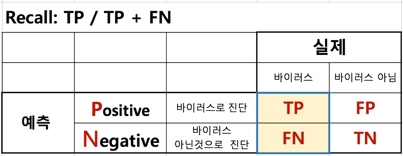
재현율(Recall)
- TP / TP + FN
참고1: numpy.linalg.svd 사용 예

In [47]:
import pandas
import numpy
import scipy.sparse
import scipy.sparse.linalg
import matplotlib.pyplot as plt
from sklearn.metrics import mean_absolute_error

data_dir = "03_data/ml-100k/"
data_shape = (943, 1682)

df = pandas.read_csv(data_dir + "ua.base", sep="\t", header=-1)
values = df.values
values[:, 0:2] -= 1
X_train = scipy.sparse.csr_matrix((values[:, 2], (values[:, 0], values[:, 1])), dtype=numpy.float, shape=data_shape)

df = pandas.read_csv(data_dir + "ua.test", sep="\t", header=-1)
values = df.values
values[:, 0:2] -= 1
X_test = scipy.sparse.csr_matrix((values[:, 2], (values[:, 0], values[:, 1])), dtype=numpy.float, shape=data_shape)

# Compute means of nonzero elements
X_row_mean = numpy.zeros(data_shape[0])
X_row_sum = numpy.zeros(data_shape[0])

train_rows, train_cols = X_train.nonzero()

# Iterate through nonzero elements to compute sums and counts of rows elements
for i in range(train_rows.shape[0]):
    X_row_mean[train_rows[i]] += X_train[train_rows[i], train_cols[i]]
    X_row_sum[train_rows[i]] += 1

# Note that (X_row_sum == 0) is required to prevent divide by zero
X_row_mean /= X_row_sum + (X_row_sum == 0)

# Subtract mean rating for each user
for i in range(train_rows.shape[0]):
    X_train[train_rows[i], train_cols[i]] -= X_row_mean[train_rows[i]]

test_rows, test_cols = X_test.nonzero()
for i in range(test_rows.shape[0]):
    X_test[test_rows[i], test_cols[i]] -= X_row_mean[test_rows[i]]

X_train = numpy.array(X_train.toarray())
X_test = numpy.array(X_test.toarray())

ks = numpy.arange(2, 50)
train_mae = numpy.zeros(ks.shape[0])
test_mae = numpy.zeros(ks.shape[0])
train_scores = X_train[(train_rows, train_cols)]
test_scores = X_test[(test_rows, test_cols)]

# Now take SVD of X_train
U, s, Vt = numpy.linalg.svd(X_train, full_matrices=False)

for j, k in enumerate(ks):
    X_pred = U[:, 0:k].dot(numpy.diag(s[0:k])).dot(Vt[0:k, :])

    pred_train_scores = X_pred[(train_rows, train_cols)]
    pred_test_scores = X_pred[(test_rows, test_cols)]

    train_mae[j] = mean_absolute_error(train_scores, pred_train_scores)
    test_mae[j] = mean_absolute_error(test_scores, pred_test_scores)

    print(k,  train_mae[j], test_mae[j])

plt.plot(ks, train_mae, 'k', label="Train")
plt.plot(ks, test_mae, 'r', label="Test")
plt.xlabel("k")
plt.ylabel("MAE")
plt.legend()
plt.show()

참고2: 다양한 추천 성능 평가 계산식 - 예: FCR
- FCP (Fraction of Concordant Pairs) : 평점이 아닌 사용자별 선호도 랭킹 기반 계산식
The RMSE metric has another issue, particularly important in our context: it assumes numerical rating values. Thus, it shares all the discussed disadvantages of such an assumption. First, it cannot express rating scales which vary among different users. Second, it cannot be applied in cases where ratings are ordinal. Thus, besides using RMSE we also employ a ranking-oriented metric which is free of the aforementioned issues.

FCP 계산 실제 코드
In [35]:
def fcp(predictions, verbose=True):
    """
    Args:
        predictions (:obj:`list` of :obj:`Prediction\
            <surprise.prediction_algorithms.predictions.Prediction>`):
            A list of predictions, as returned by the :meth:`test()
            <surprise.prediction_algorithms.algo_base.AlgoBase.test>` method.
        verbose: If True, will print computed value. Default is ``True``.
    Returns:
        The Fraction of Concordant Pairs.
    Raises:
        ValueError: When ``predictions`` is empty.
    """

    if not predictions:
        raise ValueError('Prediction list is empty.')

    predictions_u = defaultdict(list)
    nc_u = defaultdict(int)
    nd_u = defaultdict(int)

    for u0, _, r0, est, _ in predictions:
        predictions_u[u0].append((r0, est))

    for u0, preds in items(predictions_u):
        for r0i, esti in preds:
            for r0j, estj in preds:
                if esti > estj and r0i > r0j:
                    nc_u[u0] += 1
                if esti >= estj and r0i < r0j:
                    nd_u[u0] += 1

    nc = np.mean(list(nc_u.values())) if nc_u else 0
    nd = np.mean(list(nd_u.values())) if nd_u else 0

    try:
        fcp = nc / (nc + nd)
    except ZeroDivisionError:
        raise ValueError('cannot compute fcp on this list of prediction. ' +
                         'Does every user have at least two predictions?')

    if verbose:
        print('FCP:  {0:1.4f}'.format(fcp))

    return fcp
참고3: 이미지 처리에 PCA 사용 예: Olivetti faces
In [10]:
from sklearn.datasets import fetch_olivetti_faces
from sklearn.decomposition import PCA

import matplotlib.pyplot as plt
%matplotlib inline
In [11]:
faces = fetch_olivetti_faces()
print(faces.DESCR)

In [40]:
# Here are the first ten guys of the dataset
fig = plt.figure(figsize=(10, 10))
print(faces.data.size)
for i in range(10):
    ax = plt.subplot2grid((1, 10), (0, i))

    ax.imshow(faces.data[i * 10].reshape(64, 64), cmap=plt.cm.gray)
    ax.axis('off')

In [18]:
# Let's compute the PCA
pca = PCA()
pca.fit(faces.data)
Out[18]:
In [41]:
# Now, the creepy guys are in the components_ attribute.
# Here are the first ten ones:

fig = plt.figure(figsize=(10, 10))
print(pca.components_.size)
for i in range(10):
    ax = plt.subplot2grid((1, 10), (0, i))

    ax.imshow(pca.components_[i * 10].reshape(64, 64), cmap=plt.cm.gray)
    ax.axis('off')

In [39]:
# Reconstruction process

from skimage.io import imsave

face = faces.data[0]  # we will reconstruct the first face

# During the reconstruction process we are actually computing, at the kth frame,
# a rank k approximation of the face. To get a rank k approximation of a face,
# we need to first transform it into the 'latent space', and then
# transform it back to the original space

# Step 1: transform the face into the latent space.
# It's now a vector with 400 components. The kth component gives the importance
# of the kth  creepy guy
trans = pca.transform(face.reshape(1, -1))  # Reshape for scikit learn

# Step 2: reconstruction. To build the kth frame, we use all the creepy guys
# up until the kth one.
# Warning: this will save 400 png images.
fig = plt.figure(figsize=(10, 10))
for i in range(20):
    ax = plt.subplot2grid((1, 20), (0, i))
    rank_k_approx = trans[:, :i].dot(pca.components_[:i]) + pca.mean_

    ax.imshow(rank_k_approx.reshape(64, 64), cmap=plt.cm.gray)
    ax.axis('off')
