SVD (SVD와 Latent Factor 모형)
6. SVD (SVD와 Latent Factor 모형)
정방 행렬 ($n x n$) $A$에 대한 다음 식에서
$$ Av = \lambda v $$$ A \in \mathbf{R}^{M \times M} $
$ \lambda \in \mathbf{R} $
$ v \in \mathbf{R}^{M} $
위 식을 만족하는 실수 $\lambda$를 고유값(eigenvalue)
단위 벡터 $v$ 를 고유벡터(eigenvector)
라고 하며, 이를 고유 분해라고 함
- 정방 행렬이 아닌 행렬 $M$에 대해서도 고유 분해와 유사한 분해가 가능
- 이를 특이값 분해(singular value decomposition)이라고 함
- $m \times n$ 크기의 행렬 $R$은 다음과 같이 세 행렬의 곱으로 나타낼 수 있음
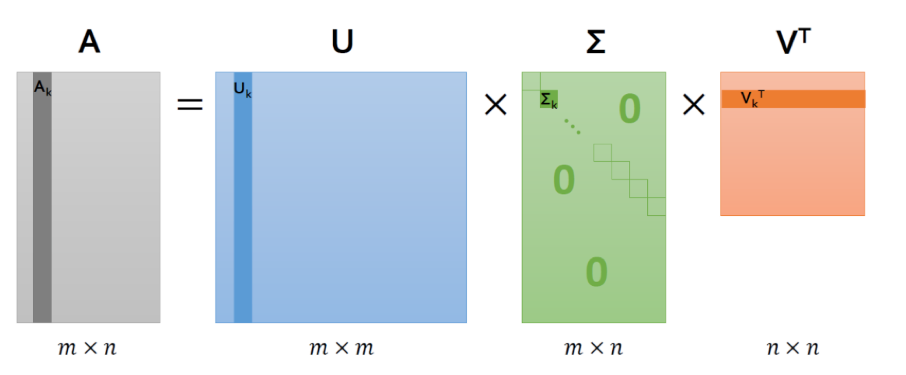
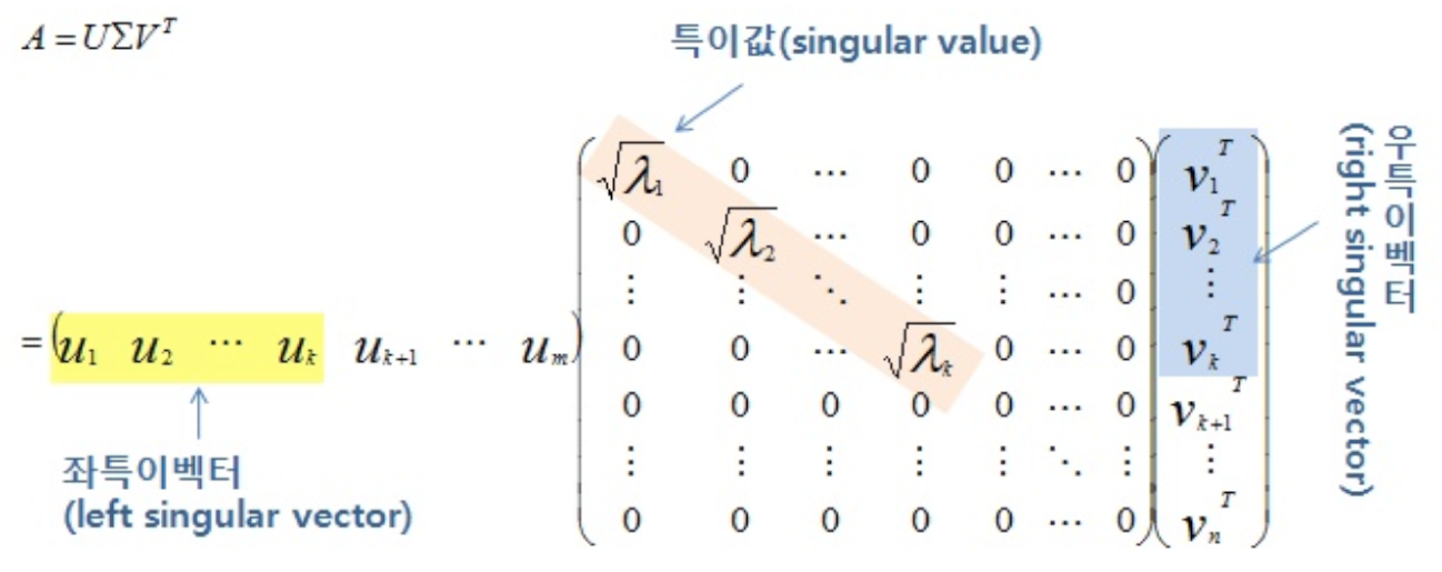
$$ R = U \Sigma V^T $$
이 식에서
- $U$ 는 $m \times m$ 크기의 행렬로 역행렬이 대칭 행렬
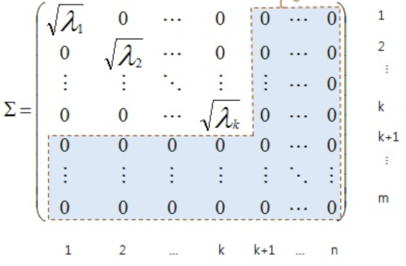
- $\Sigma$ 는 $m \times n$ 크기의 행렬로 비대각 성분이 0
- $V$ 는 $n \times n$ 크기의 행렬로 역행렬이 대칭 행렬
- V 와 U 는 직교행렬(orthogonal matrix) 특성
SVD은 R 과 RT 의 PCA
- 사용자 요인 벡터와 영화 요인 벡터로 사용자/영화별 평점 행렬의 요인 벡터로 분리하자!
* A는 SVD에 의해 $U \Sigma V^T$ 로 분해 가능 - 그렇다면, $AA^T$ = $Q \Lambda Q^T$ - 이 때 역시, $Q$:고유벡터를 열로 가지는 행렬, $\Lambda$:고유값으로 채워진 대각행렬
* SVD 수식을 사용하면, - $AA^T = (U\Sigma V^T)(U\Sigma V^T)^T = (U\Sigma V^T)(V\Sigma^T U^T) = U(\Sigma \Sigma^T)U^T$ - $A^TA = (U\Sigma V^T)^T(U\Sigma V^T) = (V\Sigma^T U^T)(U\Sigma V^T) = V(\Sigma^T \Sigma)V^T$ - V 와 U 는 직교행렬(orthogonal matrix) 특성을 가지므로, $U^T U = I$ $V^T V = I$
* 다시 행렬 A의 공분산 행렬 식을 보면,
$$\begin{align*} \Sigma =cov(A)&= \frac{1}{n-1} \sum_{i=1}^n (A_i-\mu)(A_i-\mu)^T = \frac { 1 }{ n-1 } A { A^T } \propto A A^T\\\\ \end{align*}$$ * $U$는 $AA^T$ 즉, $A$의 공분산 행렬의 고유벡터 * $V$는 $A^T A$ 즉, $A^T$의 공분산 행렬의 고유벡터 * $\Sigma \Sigma^T$ 또는 $\Sigma^T \Sigma = \lambda$ - 따라서, singular value (특이값) $σ$ = $\sqrt{\lambda}$
- 다시 행렬 A의 공분산 행렬 식을 보면,

- $\Sigma$ 는 공분산 행렬의 고유값의 제곱근(루트)
$\begin{align*} { A }^{ T }A&={ (U\Sigma { V }^{ T }) }^{ T }U\Sigma { V }^{ T }\\ &=V\Sigma { U }^{ T }U\Sigma { V }^{ T }\\ &=V{ \Sigma }^{ 2 }{ V }^{ T }\\ &=V\Lambda { V }^{ T } \end{align*}$
다시 정리 하는 SVD
- 정방행렬이 아닌 A 행렬 (m x n) 에 대해
- $U: AA^T$의 고유벡터 (m x m)
- $\Sigma : A$의 특이값들을 대각항으로 가지는 대각행렬 (m x n)
- 특이값(singular value)은 $AA^T 와 A^T A$의 고유값의 제곱근
- $V: A^T A$의 고유벡터 (n x n)
SVD은 $A$ 와 $A^T$ 의 PCA
- $ U \Sigma V^T $ 에서 $ \Sigma $ 는 대각행렬로 $ U 와 V^T $의 중복 고유값의 제곱으로 scaler 역할이 됨
- 따라서, A 행렬 = $U$ $V^T$ 로 행렬 인수분해한 모델로 가정할 수 있음
- $U$는 X (사용자 수 x k) 인 사용자 특징(요인) 행렬
- $\Sigma V^T$는 Y (영화 수 x k) 인 영화 특징(요인) 행렬
- $\Sigma$ 은 scale에 관련된 값이므로 특별히 특징 행렬로 큰 그림을 그릴시에는 무시해도 됨
이를 좀더 모델로 구체화하면

$$ r_{ui} = p_u \cdot q_i $$
- $p_u$: $U$의 한 행으로 사용자 요인을 나타냄
- $q_u$: $V^T$의 한 열로 영화 요인을 나타냄
사용자의 요인을 벡터화
\begin{array}{ll} \text{Alice} & = 10\% \color{#048BA8}{\text{ Action fan}} &+ 10\% \color{#048BA8}{\text{ Comedy fan}} &+ 50\% \color{#048BA8}{\text{ Romance fan}} &+\cdots\\ \text{Bob} &= 50\% \color{#048BA8}{\text{ Action fan}}& + 30\% \color{#048BA8}{\text{ Comedy fan}} &+ 10\% \color{#048BA8}{\text{ Romance fan}} &+\cdots\\ \text{Titanic} &= 20\% \color{#048BA8}{\text{ Action}}& + 00\% \color{#048BA8}{\text{ Comedy}} &+ 70\% \color{#048BA8}{\text{ Romance}} &+\cdots\\ \text{Toy Story} &= 30\% \color{#048BA8}{\text{ Action }} &+ 60\% \color{#048BA8}{\text{ Comedy}}&+ 00\% \color{#048BA8}{\text{ Romance}} &+\cdots\\ \end{array}
\begin{align*} p_\text{Alice} &= (10\%,~~ 10\%,~~ 50\%,~~ \cdots)\\ p_\text{Bob} &= (50\%,~~ 30\%,~~ 10\%,~~ \cdots)\\ q_\text{Titanic} &= (20\%,~~ 00\%,~~ 70\%,~~ \cdots )\\ q_\text{Toy Story} &= (30\%,~~ 60\%,~~00\%,~~ \cdots ) \end{align*}

\begin{align*} r_{ui}= p_u \cdot q_i = \sum_{f \in \text{latent factors}} \text{affinity of } u \text{ for } f \times \text{affinity of } i \text{ for }f \end{align*}
import numpy as np
from numpy import linalg as la
np.random.seed(42)


def flip_signs(A, B):
    """
    utility function for resolving the sign ambiguity in SVD
    http://stats.stackexchange.com/q/34396/115202
    """
    signs = np.sign(A) * np.sign(B)
    return A, B * signs


# Let the data matrix X be of n x p size,
# where n is the number of samples and p is the number of variables
n, p = 5, 3
X = np.random.rand(n, p)
# Let us assume that it is centered
# 평균이 0으로 맞춘 후에 (centering 작업 수행) 공분산 행렬을 계산함
X -= np.mean(X, axis=0)

# the p x p covariance matrix
C = np.cov(X, rowvar=False)
print ("covariance matrix = \n", C)
# C is a symmetric matrix and so it can be diagonalized:
l, principal_axes = la.eig(C)
# sort results wrt. eigenvalues
idx = l.argsort()[::-1]
l, principal_axes = l[idx], principal_axes[:, idx]
# the eigenvalues in decreasing order
print ("eigenvalues = \n", l)
# a matrix of eigenvectors (each column is an eigenvector)
print ("eigenvectors = \n", principal_axes)
# projections of X on the principal axes are called principal components
principal_components = X.dot(principal_axes)
print ("principal_components = \n", principal_components)

# we now perform singular value decomposition of X
# "economy size" (or "thin") SVD
U, s, Vt = la.svd(X, full_matrices=False)
V = Vt.T
S = np.diag(s)

# 1) then columns of V are principal directions/axes.
print ("V = \n", V)
assert np.allclose(*flip_signs(V, principal_axes))

# 2) columns of US are principal components
print ("US = \n", U.dot(S))
assert np.allclose(*flip_signs(U.dot(S), principal_components))

# 3) singular values are related to the eigenvalues of covariance matrix
print ((s ** 2) / (n - 1))
assert np.allclose((s ** 2) / (n - 1), l)

# 8) dimensionality reduction
k = 2
PC_k = principal_components[:, 0:k]
US_k = U[:, 0:k].dot(S[0:k, 0:k])
print (US_k)
assert np.allclose(*flip_signs(PC_k, US_k))

print (U)
print (S)
print (V)
# 10) we used "economy size" (or "thin") SVD
assert U.shape == (n, p)
assert S.shape == (p, p)
assert V.shape == (p, p)
특이값 분해 계산
import numpy as np
from pprint import pprint
import math
M = np.array([[math.sqrt(3), 2], [0, math.sqrt(3)]])
U, s, Vt = numpy.linalg.svd(M, full_matrices=True)
M
- $A^T A$ 의 고유값: $\lambda_1 = 9$, $\lambda_2 = 1$
- 특이값: $σ_1$ = $\sqrt{\lambda_1}$ = 3, $σ_2$ = $\sqrt{\lambda_2}$ = 1
- $\lambda_1 = 9$ 에 대응하는 $A^T A$의 단위고유벡터는 $v_1 = \begin{pmatrix} \frac{1}{2} \\ \frac{\sqrt{3}}{2} \end{pmatrix}$
- $\lambda_2 = 1$ 에 대응하는 $A^T A$의 단위고유벡터는 $v_2 = \begin{pmatrix} -\frac{\sqrt{3}}{2} \\ \frac{1}{2} \end{pmatrix}$
- $u_1 = \frac{1}{σ_1}Av_1 = \begin{pmatrix} \frac{\sqrt{3}}{2} \\ \frac{1}{2} \end{pmatrix}$
- $u_2 = \frac{1}{σ_2}Av_2 = \begin{pmatrix} -\frac{1}{2} \\ \frac{\sqrt{3}}{2} \end{pmatrix}$
- $U = [u_1, u_2] = \begin{pmatrix} \frac{\sqrt{3}}{2} \ -\frac{1}{2} \\ \frac{1}{2} \ \frac{\sqrt{3}}{2} \end{pmatrix}$
U
- $V^T = [v_1, v_2] = \begin{pmatrix} \frac{1}{2} \ \frac{\sqrt{3}}{2} \\ -\frac{\sqrt{3}}{2} \ \frac{1}{2}\end{pmatrix}$
Vt
$ \Sigma = \begin{pmatrix} 3 \ 0 \\ 0 \ 1 \end{pmatrix}$
np.diag(s)
$ U \Sigma V^T = \begin{pmatrix} \frac{\sqrt{3}}{2} \ -\frac{1}{2} \\ \frac{1}{2} \ \frac{\sqrt{3}}{2} \end{pmatrix} \begin{pmatrix} 3 \ 0 \\ 0 \ 1 \end{pmatrix}\begin{pmatrix} \frac{1}{2} \ \frac{\sqrt{3}}{2} \\ -\frac{\sqrt{3}}{2} \ \frac{1}{2}\end{pmatrix}$
U.dot(np.diag(s)).dot(Vt)
import numpy as np
from pprint import pprint
M = np.array([[1,0,0,0,0],[0,0,2,0,3],[0,0,0,0,0],[0,2,0,0,0]])
U, S0, V0 = np.linalg.svd(M, full_matrices=True)
M
U
S0
S = np.hstack([np.diag(S0), np.zeros(M.shape[0])[:, np.newaxis]])
S
V = V0.T
V
print("\nU.dot(S).dot(V.T):"); pprint(U.dot(S).dot(V0))
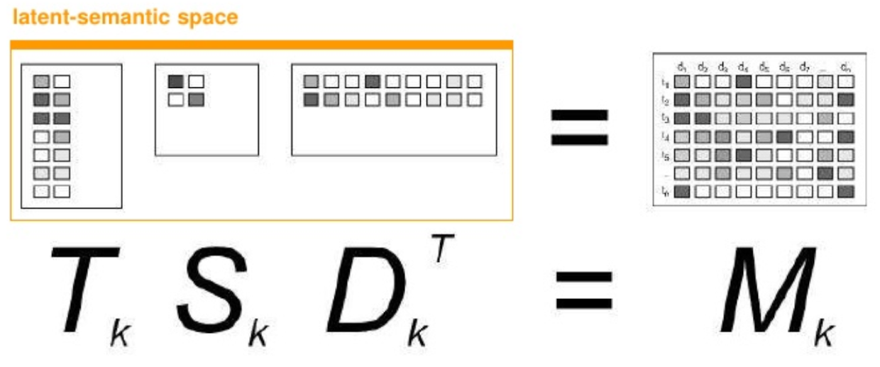
Trancated SVD: S에서 고유값 제곱이 0인 부분들을 없애면 차원 축소가 가능하고, 계산량을 줄일 수 있음
계산량 축소 $\lambda > 0$ 인 것만 사용하기
S
sklearn의 TruncatedSVD 사용 예
from sklearn.decomposition import TruncatedSVD
from sklearn.random_projection import sparse_random_matrix
X = sparse_random_matrix(5, 5)
svd = TruncatedSVD(n_components=2, n_iter=7)
U = svd.fit_transform(X)
Sigma = svd.explained_variance_ratio_
VT = svd.components_
svd.fit(X)
U
- 나머지 singular vector value는 0이기 때문에 삭제한다.
Sigma
VT
- 본래 U는 5X5, Sigma는 5X5, $V^T$는 5X5
- Truncated SVD로 변환: U는 5X2, Sigma는 2X2, $V^T$는 2X5
그러나, 사실 PCA, SVD는 dense matrix에서나 가능한 예!
- SVD는 dense matrix인 이미지의 차원축소에 많이 사용됨
- 사용자/영화의 평점 행렬은 평점이 많지 않은 sparse 행렬임!
어떻게 sparse 행렬인 사용자/영화 평점 행렬에 SVD를 사용할까?
- 초기 $p_u$, $q_u$를 임의로 정하고, 이를 이용해서 근사 행렬 $Q$를 구한다.
$$ r_{ui} = p_u \cdot q_i $$
- $p_u$: $U$의 한 행으로 사용자 요인을 나타냄
- $q_u$: $V^T$의 한 열로 영화 요인을 나타냄
어떻게 사용자, 영화 특징(요인)으로부터 계산된 예측 평점의 정확도를 높일 것인가?
- $r_{ui}$ 를 $Q$라 하고, 실제 평점 $R$과의 차이를 손실 함수로 만들자
- min($R$ - $Q$)
sparse matrix인 평점 행렬에 대해 SGD를 사용한 실제 SVD 구현 예
import numpy as np
import surprise  # run 'pip install scikit-surprise' to install surprise
class SVD_SGD(surprise.AlgoBase):

    def __init__(self, learning_rate, n_epochs, n_factors):

        self.lr = learning_rate  # learning rate for SGD
        self.n_epochs = n_epochs  # number of iterations of SGD
        self.n_factors = n_factors  # number of factors (몇 개의 Latent Factor로 요인 벡터를 만들지를 정함)

    def train(self, trainset):
        '''Learn the vectors p_u and q_i with SGD'''

        print('Fitting data with SGD...')

        # Randomly initialize the user and item factors.
        p = np.random.normal(0, .1, (trainset.n_users, self.n_factors))
        q = np.random.normal(0, .1, (trainset.n_items, self.n_factors))

        # SGD procedure
        for _ in range(self.n_epochs):
            for u, i, r_ui in trainset.all_ratings():
                err = r_ui - np.dot(p[u], q[i])
                # Update vectors p_u and q_i
                p[u] += self.lr * err * q[i]
                q[i] += self.lr * err * p[u]
                # Note: in the update of q_i, we should actually use the previous (non-updated) value of p_u.
                # In practice it makes almost no difference.

        self.p, self.q = p, q
        self.trainset = trainset

    def estimate(self, u, i):
        '''Return the estmimated rating of user u for item i.'''

        # return scalar product between p_u and q_i if user and item are known,
        # else return the average of all ratings
        if self.trainset.knows_user(u) and self.trainset.knows_item(i):
            return np.dot(self.p[u], self.q[i])
        else:
            return self.trainset.global_mean
# data loading. We'll use the movielens dataset (https://grouplens.org/datasets/movielens/100k/)
# it will be downloaded automatically.
data = surprise.Dataset.load_builtin('ml-100k')
data.split(2)  # split data for 2-folds cross validation
algo = SVD_SGD(learning_rate=.01, n_epochs=10, n_factors=10)
surprise.evaluate(algo, data, measures=['RMSE'])
베이스라인 모형(baseline model)을 사용해서 sparse 행렬에 미리 값을 넣은 후에 SGD를 돌리는 방식도 가능
사용자 아이디 $u$, 상품 아이디 $i$, 두 개의 카테고리 값 입력에서 평점 $r_{ui}$의 예측치 $\hat{r}_{ui}$ 을 예측하는 단순 모형
사용자와 상품 특성에 의한 평균 평점의 합으로 나타난다.
$$ \hat{r}_{ui} = \mu + b_u + b_i $$$\mu$는 전체 평점의 평균
$b_u$는 동일한 사용자에 의한 평점 평균값
$b_i$는 동일한 상품에 대한 평점 평균값